Posts

Excel - Solver examples
Image
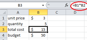
Excel Solver is used to solve optimization problems, which is like solving equations. In this tutorial, we will give a very simple example on how to use Excel Solver. Basic example Suppose your car is low on gasoline. The gasoline is $3/gallon. You have a budget of $50. How much gasoline can you buy? Of course, for a problem this simple, we do not even need a Solver to solve the problem. However, the purpose is to teach the users how to use Excel Solver, so we make the problem extremely simple. We have the following framework: Goal: maximize quantity of gasoline Relationship: cost=quantity * unit price Constraint: cost<=budget 1. In cell B1, we enter unit price "3", in cell B4, we enter the budget 50. In cell B2, we just enter an arbitrary number as the number of gallons. We entered 5. In cell B3, we enter the formula "=B1*B2" to let it be the cost, which equals to 15. 2. Click Solver under the Data menu. 3. A Solver dialog window pops up. In "Set objective&

Excel - How to count the number of sign changes (from + to - or vice versa) in a column?

Image
Suppose you have a column of numbers and the data can be positive or negative. How do you count the number of times the data changes from positive to negative, or vice versa? We will use three functions, SIGN , INT and SUM to solve the problem. First we add a helper column B, name it "sign", then use SIGN function to get its sign. If the data is positive, it returns 1. If the value is negative, it returns -1. The formula is like: =SIGN(A2) Then we add another helper column C, call it "sign change", which checks whether sign of the current value is different from the last value. INT function is used to return the logical value TRUE or FALSE into 1 or 0. At last, at the end of column C, we use a SUM function to sum all the value changes. In this example, the data sign changes for 4 times (-1 to -3, -3 to 4, 2 to -5, and -5 to 6). VBA method Below is the VBA code to achieve it. You need to add a clickable button on the spreadsheet and assign the following code t

Excel - Convert between mile, kilometer and meter

Image
Excel has a very useful function convert numbers from one measure unit to another, for example, from Fahrenheit to Celsius, or from mile to kilometer. The function is  CONVERT . For example, if we want to convert temperature 1.2 mile to kilometer, how to do it? One way is using the equation: 1 mile = 1.60934 kilometer If you do not know the conversion equation, you can just use the CONVERT function. Since kilometer is not a basic unit in the CONVERT function, you need to convert mile into meter first and then to kilometer. For example: =CONVERT(1.2,"mi","m") will turn mile into meters. If you divided the above number by 1000, you will get kilometer. =CONVERT(1.2,"mi","m")/1000 See the following figure for example. You can also convert kilometer into mile in a similar way. You first need to convert kilometer into meter, then use the CONVERT function. The formula is: =CONVERT(2.35*1000,"m","mi")

Excel - How to convert Fahrenheit to Celsius

Image
Excel has a very useful function convert numbers from one measure unit to another, for example, from Fahrenheit to Celsius, or from mile to kilometer. The function is CONVERT . For example, if we want to convert temperature 76 F to Celsius, how to do it? One way is using the equation: C=(F-32)/1.8 If you do not know the conversion equation, you can just use the CONVERT function. For example: =CONVERT(76,"F","C") In the following figure, both methods give the same result.

Google Sheets - YEARFRAC function

Image
YEARFRAC function returns the number of fractional years between two days. Syntax YEARFRAC( start_date, end_date, [day_count_convention] ) The day_count_convention is optional and will be ignored in this tutorial. Examples The above result shows that there is 0.497 year between 1/1/2020 and 6/30/2020, or the duration between 1/1/2020 and 6/30/2020 is 49.72%.

Google Sheets - YEAR function

Image
YEAR function returns the year part of a date. For example, the year part of 2/20/2020 is 2020. Syntax YEAR(date) Examples

Google Sheets - WORKDAY.INTL function

Image
The WORKDAY  function answers questions like this: what date is it after 15 work days from 1/3/2020? WORKDAY function assumes that Saturday and Sunday are not work days. However, in some countries, the rest days may be Sunday and Monday. WORKDAY.INTL solve this problem. Syntax WORKDAY( date, number of work days, [weekend], [holidays] ) weekend is optional. weekend is a string of seven 0s and 1s, representing seven days from Monday to Sunday. 0 indicates work days and 1 indicates rest days. The default is "0000011", which means Monday to Friday are work days, while Saturday and Sunday are not weekend. If Sunday and Monday are rest days while Tuesday to Saturday are work days, we should use "1000001". Holidays  are optional If  number of work  days is negative, we calculate like what date it is 3 work days before this date Examples In the above example, it shows that 25 work days after 1/2/2020 is 2/13/2020 in China.