Blog of Calc LLC

Excel has a very useful function convert numbers from one measure unit to another, for example, from Fahrenheit to Celsius, or from mile to kilometer. The function is  CONVERT . For example, if we want to convert temperature 1.2 mile to kilometer, how to do it? One way is using the equation: 1 mile = 1.60934 kilometer If you do not know the conversion equation, you can just use the CONVERT function. Since kilometer is not a basic unit in the CONVERT function, you need to convert mile into meter first and then to kilometer. For example: =CONVERT(1.2,"mi","m") will turn mile into meters. If you divided the above number by 1000, you will get kilometer. =CONVERT(1.2,"mi","m")/1000 See the following figure for example. You can also convert kilometer into mile in a similar way. You first need to convert kilometer into meter, then use the CONVERT function. The formula is: =CONVERT(2.35*1000,"m","mi")

If you make an investment and the returns are paid to you periodically, you can use NPV function to calculate NPV of the investment. What if the returns are paid to you not periodically? You will need XNPV function. You can think "X" in XNPV as "special". So XNPV function is a special type of NPV function. Suppose you make an investment on January 1, 2020, and the returns are paid to you on specific days, like below. XNPV function can be used. The formula is: =XNPV(B1, B4:B7, A4:A7) B1 is the rate, B4:B7 are the cash flows, and A4:A7 are the dates you receive the cash.

NPV function calculates the net present value of a future positive or negative cash flows. For example, suppose you will receive an income of $100 one year later, how much does it worth today? $100 received one year later worth less than $100 received today. Because if you have $100 in hand at this moment and invest it, suppose the return rate is 5%, then it will grow into $105 one year later. Next, we will show you how to calculate the net prevent value of $100 received one year later. Let the net prevent value of $100 received one year later be X, and suppose the investment return rate is 5%. Then X*(1+0.05)=$100 So, X=$100/(1+0.05)=$95.24 It means that if you have $95.25 in hand right now and invest it with 5% investment return, it will grow into $100 one year later. Therefore, $100 received one year later is worth $95.24 today. That is to say, the net prevent value (NPV) of $100 received one year later is $95.24. If you use NPV function, the formula is: =NPV(0.05, 100) What is the ...

SUM function calculate the sum of a range of numbers. The formula is: =SUM(B2:B5)

Unlike most other Excel functions which deal with a single number, a row or a column, INDEX function deals with a data table. It answers questions such as "what is the number at row 3 and column 4?" In the data range highlighted yellow above, what is the number at row 3 and column 2? Remember we only talk about the data range, not including header row. So the data on row 3 is carrot, not banana. The formula is: =INDEX(A2:B5,3,2) It returns 1.5, which is the price of carrot.

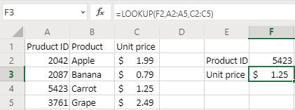
If you do not know the meaning of a word, you can take out a dictionary and look up the word and get the meaning. Excel LOOKUP function does the similar thing. For example, you do not know the price associated with a product ID, you can use LOOKUP function to retrieve the price. Suppose you own a grocery store. You remember the product ID of carrot is 5423, but you do not remember the price. A LOOKUP function can help you. The formula is: =LOOKUP(F2, A2:A5, C2;C5) You enter the product ID in cell F2. It looks for the value in the data range of A2:A5, the return the corresponding value in data range C2:C5. For example, the product ID of 5423 is on row 4, the the unit price for row 4 is $1.25. Note: VLOOKUP is an improved version of LOOKUP. So use VLOOKUP instead of LOOKUP if possible.

The DAYS function returns the difference between two days. =DAYS(C2, B2) For example, the number of days between "7/8/2019" and "1/28/2020" is 204. Internally, Excel convert date value into integers and subtract these two integers. Excel store "7/28/2019" as 43654 and store "1/28/2020" as 43858. And 43858-43654=204, giving the same result as using the DAYS function. Note: The DAYS function needs two arguments, the first one is the end date, the second one is the start date. It is counter-intuitive for many people and different from many other data software, so be very careful.

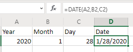
DATE function generate a date from year, month and day. For example: =DATE (A2, B2, C2) Note: 1. If the date is shown as numbers, like below, you need to format it as date. 2. Always use four digit years such as 1978 or 2020. If you use two-digit years such as 20, it may not be what you want.

If you have a range of values, MATCH function finds the position in the range of a value given by you. For example, if you are studying a population and have age groups like below, which age group does age 16 belongs to? =MATCH(16, A2:A10, 1) The third argument 1 is the default value, and is optional. It is equivalent to the following formula in this example. =MATCH(16, A2:A10) There are 9 numbers from 0 to 80. The returned value is 3, which means the 3rd number in the list. It means age 16 belongs to the 13 to 17 age group. The row number of 13 is 4, but 13 is the 3rd number in the list, so the returned value is 3, not 4. Tip: The MATCH position only returns the relative position in a list of values, not the age group name such as "13 to 17". To return the age group name, use LOOKUP function instead. To do exact matching: The values can be in any order. But the third argument has to be 0, like below: =MATCH(16, A2:A10, 0) If the data is ordered from large to small, the third...

If you have a list of values, Excel CHOOSE functions returns a certain value by the index number. For example, if you have the week days from Monday to Sunday, the 2nd one is Tuesday. Note: When using CHOOSE function, you cannot select a data range such as A2:A8, you have to select the values one by one, separated by comma. The formula is: =CHOOSE(D2,A2,A3,A4,A5,A6,A7,A8) You can manually enter values instead of cell positions. For example, the following formula returns "banana". =CHOOSE(2,"apple","banana","orange")

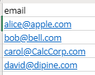
FIND returns the position of one text string in another text string. For example, you may want to know position of "@" in an email address. If we know position of "@" in an email address, we can further extract the domain name of an email address. Suppose you have a list of email addresses below. 1. Find position of "@" in the email address. The formula is: =FIND("@", A2) For example, "@" is the 6th character in the "alice@apple.com", so it returns a value of 6. 2. Calculate length of email address, the LEN function is used. =LEN(A2) 3. Based on length of an email address and position of "@" in it, we use MID function to extract the domain name. =MID(A2, B2+1, C2-B2) "B2+1" is the first character after the "@" sign, which is 7 in the first email address. "C2-B2" is the number of characters after the "@", which is 9 in the first email address. The MID function reads the emai...

If function is a logic function. It does two things: Whether the criteria is met Return a value based on whether the criteria is met or not. If the criteria is met, it returns one value; if the criteria is not met, it returns a different value. The reason IF function is confusing for some Excel users is that it does two things: a logical test, AND a return value depending on the logical test result, while the name of "IF" implies it only does a logical test. If this function only returns TRUE or False, it would be much easier to understand. In the following example, there are 5 employees, each having his own budget. Column C records the exact amount of money they spent. If the actual spending is greater than budget, we call it "Over budget", otherwise, we call it "Within budget". The IF function is: =IF(C2>B2,"Over budget","Within budget") The first part, "C2>B2", is a logical test. If this is TRUE, then the IF function ...

Suppose you have a problem like below, how are you going to solve it? If score of a student is 90 or above, set the grade to A; Else if the score is 80 or above, set the grade to B; Else if the score is 70 or above, set the grade to C; Else if the score is 60 or above, set the grade to D; Else set the grade to F. In the past, you will have to write nested IF functions. But now there is new Excel function IFS, which can solve the problem easily. To help you remember the IFS function, you can think it as the plural form of IF function, just like "apple" vs "apples". The formula is: =IFS(B2>90,"A",B2>80,"B",B2>70,"C",B2>60,"D", TRUE,"F" ) The last 2 items in the formula [ True, "False" ] set the default value. It means that, if none of the previous criteria is met, it will return the value of "F". You do not have to set the default value, but then you need to include all the possible valu...

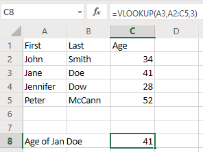
This post is written by Yisong Geng, PhD at Calc LLC. If you need consulting services with Excel, please  contact us . VLOOKUP is one of the most commonly used Excel functions. VLOOKUP function asks for 4 things: The value you want to look up, such as name of a person The data range you want to search If the value is found in the data range, which column contains the value you want the function to return? Whether it is a approximate match or not. The default option is approximate match. This argument is optional and let's ignore it for now. The following table contains first name, last name and age of 4 people. Your task is to find the age of Jan Doe. It can be easily done using VLOOKUP function. The value you want to look up is "Jane", which is at cell "A3" The range of data you want to search, which is "A2:C5" Which column contains the value you want to retrieve? The "Age" is column C, so this argument is 3. The 4th argument is optional and...

ACOS function returns arccosine, or inverse of cosine function, of a number. For example, the cosine of pi/3 (or 60 degrees) is 0.5. Therefore, arccosine of 0.5 is pi/3 (or 60 degrees).

ABS function returns the absolute value of a number.