Excel Solver is used to solve optimization problems, which is like solving equations. In this tutorial, we will give a very simple example on how to use Excel Solver.
We have the following framework:
Goal: maximize quantity of gasoline
Relationship: cost=quantity * unit price
Constraint: cost<=budget
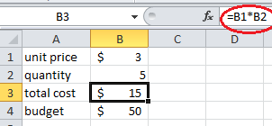
1. In cell B1, we enter unit price "3", in cell B4, we enter the budget 50. In cell B2, we just enter an arbitrary number as the number of gallons. We entered 5. In cell B3, we enter the formula "=B1*B2" to let it be the cost, which equals to 15.


6. It tells you the Solver found a solution. Click OK.


We have the following framework:
Relationship: cost=quantity * unit price
Goal: maximize quantity of gasoline
Constraint 1: cost<=budget
Constraint 2: quantity should be integer
1. Add a constraint to let cell $B$2 be integer

2. The solver parameter dialog window look like this. Click Solve.

3. Now the optimized quantity is 16, which means you can buy up to 16 apples with $50.


The numbers in range B11:D13 can only be 0 or 1, which is called "binary". In the following constraint, we require them to be binary.


The result shows that the area is maximized when lengths of all sides equal to 5, which is a square.


2. Add some cells indicating the number of times we leave or enter a note. The Outflow column records the number of times we leave this node. The Inflow column indicates the number of times we enter a node. The outflow-inflow column measures the difference between the number of times we leave and enter a node. The formula for outflow at node S, for example, is:
=SUMIF(FROM,G2,TAKE_OR_NOT)
The formula for inflow at node E is:
=SUMIF(TO,G7,TAKE_OR_NOT)
FROM is a name for range A2:A25, TO is a name for range B2:B25. DISTANCE is a name for range C2:C25. TAKE_OR_NOT is a name for range E2:E25.

3. Here are the Solver Parameters. We want to minimize cell C26 (total distance), by changing cells in TAKE_OR_NOT (meaning whether we take a path or not). Constraint "J2=1" means we leave node S (start point) for once (in net). Constraint J8= -1 means we enter node T (terminal point) for once. The range J3:J7 should be 0 means for nodes A to E, if we enter a node for one time, we should also leave that node for one time.


The red path in the following graph shows the shortest path. The total distance is 3+3+4=10, same as what the Solver told us.

Basic example
Suppose your car is low on gasoline. The gasoline is $3/gallon. You have a budget of $50. How much gasoline can you buy? Of course, for a problem this simple, we do not even need a Solver to solve the problem. However, the purpose is to teach the users how to use Excel Solver, so we make the problem extremely simple.We have the following framework:
Goal: maximize quantity of gasoline
Relationship: cost=quantity * unit price
Constraint: cost<=budget
1. In cell B1, we enter unit price "3", in cell B4, we enter the budget 50. In cell B2, we just enter an arbitrary number as the number of gallons. We entered 5. In cell B3, we enter the formula "=B1*B2" to let it be the cost, which equals to 15.
2. Click Solver under the Data menu.
3. A Solver dialog window pops up. In "Set objective" we enter "$B$2", which is the quantity of gasoline that we want to maximize. In "By Changing Variable Cells", we also enter "$B$2", since this is the only thing we can change. Then click "Add" to add constraints.
4. In the constraint, we require "$B$3"<="$B$4". Then click OK.
5. Now you see the following window. The Solver is ready to work. Click Solve.
7. Now the value of cell "B2" changes to 16.66667. The cost is exactly $50. It means that with total budget of $50, you can buy up to 16.66667 gallons of gasoline.
Integer constraint
Now let's change the question a little bit. Suppose you want to buy some apples. The apple costs $3 each. You have a budget of $50. How many apples can you buy? The question is almost identical to the above gasoline question, except that the number of apples has to be integers such as 3 or 5, but not 3.7 or 8.2.We have the following framework:
Relationship: cost=quantity * unit price
Goal: maximize quantity of gasoline
Constraint 1: cost<=budget
Constraint 2: quantity should be integer
1. Add a constraint to let cell $B$2 be integer
Multiple items and multiple constraints
Now we work on a little bit more complex issue. Suppose you run a computer store. You sell two products: computer and monitor. You have two constraints: budget and store storage space. The question is how many computers and monitors should you order so that the profit is maximized?
Look at the numbers on the left in the following figure. If you sell a computer and monitor, the profit is $300 and $50 respectively. The capital needed to buy a computer and monitor is $1200 and $150 respectively. The storage space needed for a computer and monitor is 1 and 0.5 respectively. Your total available budget is $24,532. Your total available storage space is 53.2. Your goal is to maximize profit. Let n1 be number of computers to order, and n2 be number of monitors to order, we have the following:
Goal: maximize profit
- profit=300*n1+50*n2
Constraints:
- 1200*n1+150*n2<=24532
- 1*n1+0.5*n2<=53.2
- n1 is integer
- n2 is inreger
After all is set up, the Solver tells us we should order 10 computers and 83 monitors. The total profit will be $7150.
Minimizing shipping cost
In this example, we show how to optimize by minimizing some numbers.
Suppose a company has 3 factories with supply capacity of 80, 250 and 270 items each. The company has 3 customers, with demand of 200, 100 and 300 items each. The total supply is 600, which is same as the total demand.
The cost of shipping from each factory to each customer varies, as shown in the following figure. Our goal is to minimize the shipping cost, which is cell G14.
Add the following constraints, which basically states that items shipped from a factory equals to its supply capacity. Items shipped to a customer equals to its demand. We also require the number of items shipped to be integer.
The result is below. The best shipping cost is $26,620.
Assignment problem
Suppose you have 3 customers needs machine maintenance services. You have 3 staff. You want to assign one staff to one customer. The travelling cost from each staff's residency to customers varies, as shown below. Your goal is to minimizing the travelling cost for your staff. This example is very similar to the above shipping cost problem, except that one staff can only serve one customer.
The numbers in range B11:D13 can only be 0 or 1, which is called "binary". In the following constraint, we require them to be binary.
And we want to minimize here. We also want the supply and demand match.
Here is the result.
Geometry
Suppose there is a rectangle. The perimeter has to be 20. What are the lengths of the sides so that the area is maximized?
In the following figure, length of side A is B1, length of side B is B2, and the perimeter is 2*(B1+B2).
Here is how the solver parameters are set.
The result shows that the area is maximized when lengths of all sides equal to 5, which is a square.
Shortest path
Excel solver can also solve problems such as shortest path in a graph, like below. Suppose you are at S (start) and you want to arrive at T (terminal). The distance from one node to another is shown. For example, the distance between A and B is 3. What is the shortest path from S to T?
1. First, we need to turn the graph into a table like below. We add a column "Take or not" to indicate whether we take the path. 1 means we take the path and 0 means not. Just initialize this column with 0.
2. Add some cells indicating the number of times we leave or enter a note. The Outflow column records the number of times we leave this node. The Inflow column indicates the number of times we enter a node. The outflow-inflow column measures the difference between the number of times we leave and enter a node. The formula for outflow at node S, for example, is:
=SUMIF(FROM,G2,TAKE_OR_NOT)
The formula for inflow at node E is:
=SUMIF(TO,G7,TAKE_OR_NOT)
FROM is a name for range A2:A25, TO is a name for range B2:B25. DISTANCE is a name for range C2:C25. TAKE_OR_NOT is a name for range E2:E25.
3. Here are the Solver Parameters. We want to minimize cell C26 (total distance), by changing cells in TAKE_OR_NOT (meaning whether we take a path or not). Constraint "J2=1" means we leave node S (start point) for once (in net). Constraint J8= -1 means we enter node T (terminal point) for once. The range J3:J7 should be 0 means for nodes A to E, if we enter a node for one time, we should also leave that node for one time.
4. Click Solve and you get the following result. We should take path S-C-E-T, with total distance of 10.
The following table shows we leave node S, enter and leave node C, enter and leave node E, and enter node T.
The red path in the following graph shows the shortest path. The total distance is 3+3+4=10, same as what the Solver told us.
Comments
Post a Comment