Blog of Calc LLC

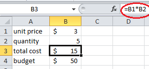
Excel Solver is used to solve optimization problems, which is like solving equations. In this tutorial, we will give a very simple example on how to use Excel Solver. Basic example Suppose your car is low on gasoline. The gasoline is $3/gallon. You have a budget of $50. How much gasoline can you buy? Of course, for a problem this simple, we do not even need a Solver to solve the problem. However, the purpose is to teach the users how to use Excel Solver, so we make the problem extremely simple. We have the following framework: Goal: maximize quantity of gasoline Relationship: cost=quantity * unit price Constraint: cost<=budget 1. In cell B1, we enter unit price "3", in cell B4, we enter the budget 50. In cell B2, we just enter an arbitrary number as the number of gallons. We entered 5. In cell B3, we enter the formula "=B1*B2" to let it be the cost, which equals to 15. 2. Click Solver under the Data menu. 3. A Solver dialog window pops up. In "Set objective...

Suppose you have a column of numbers and the data can be positive or negative. How do you count the number of times the data changes from positive to negative, or vice versa? We will use three functions, SIGN , INT and SUM to solve the problem. First we add a helper column B, name it "sign", then use SIGN function to get its sign. If the data is positive, it returns 1. If the value is negative, it returns -1. The formula is like: =SIGN(A2) Then we add another helper column C, call it "sign change", which checks whether sign of the current value is different from the last value. INT function is used to return the logical value TRUE or FALSE into 1 or 0. At last, at the end of column C, we use a SUM function to sum all the value changes. In this example, the data sign changes for 4 times (-1 to -3, -3 to 4, 2 to -5, and -5 to 6). VBA method Below is the VBA code to achieve it. You need to add a clickable button on the spreadsheet and assign the following code t...

Excel has a very useful function convert numbers from one measure unit to another, for example, from Fahrenheit to Celsius, or from mile to kilometer. The function is  CONVERT . For example, if we want to convert temperature 1.2 mile to kilometer, how to do it? One way is using the equation: 1 mile = 1.60934 kilometer If you do not know the conversion equation, you can just use the CONVERT function. Since kilometer is not a basic unit in the CONVERT function, you need to convert mile into meter first and then to kilometer. For example: =CONVERT(1.2,"mi","m") will turn mile into meters. If you divided the above number by 1000, you will get kilometer. =CONVERT(1.2,"mi","m")/1000 See the following figure for example. You can also convert kilometer into mile in a similar way. You first need to convert kilometer into meter, then use the CONVERT function. The formula is: =CONVERT(2.35*1000,"m","mi")

Excel has a very useful function convert numbers from one measure unit to another, for example, from Fahrenheit to Celsius, or from mile to kilometer. The function is CONVERT . For example, if we want to convert temperature 76 F to Celsius, how to do it? One way is using the equation: C=(F-32)/1.8 If you do not know the conversion equation, you can just use the CONVERT function. For example: =CONVERT(76,"F","C") In the following figure, both methods give the same result.

If you make an investment and the returns are paid to you periodically, you can use NPV function to calculate NPV of the investment. What if the returns are paid to you not periodically? You will need XNPV function. You can think "X" in XNPV as "special". So XNPV function is a special type of NPV function. Suppose you make an investment on January 1, 2020, and the returns are paid to you on specific days, like below. XNPV function can be used. The formula is: =XNPV(B1, B4:B7, A4:A7) B1 is the rate, B4:B7 are the cash flows, and A4:A7 are the dates you receive the cash.

NPV function calculates the net present value of a future positive or negative cash flows. For example, suppose you will receive an income of $100 one year later, how much does it worth today? $100 received one year later worth less than $100 received today. Because if you have $100 in hand at this moment and invest it, suppose the return rate is 5%, then it will grow into $105 one year later. Next, we will show you how to calculate the net prevent value of $100 received one year later. Let the net prevent value of $100 received one year later be X, and suppose the investment return rate is 5%. Then X*(1+0.05)=$100 So, X=$100/(1+0.05)=$95.24 It means that if you have $95.25 in hand right now and invest it with 5% investment return, it will grow into $100 one year later. Therefore, $100 received one year later is worth $95.24 today. That is to say, the net prevent value (NPV) of $100 received one year later is $95.24. If you use NPV function, the formula is: =NPV(0.05, 100) What is the ...

Similar to treemap chart, sunburst chart is also used to show hierarchical data. For example, suppose you run a factory and your products are sold all around the world. The following shows your market and number of machines sold in each market. 1. Select the data. Click Insert > Charts > Other Charts. Under Hierarchical, select Sunburst. 2. Now you get a sunburst chart. The inner most circle shows the highest level of data, while the outer most circle shows the finest level of data.

Pareto chart shows relative importance of each factor to the total. It it is used to show which factors are more important and which factors are less important. Suppose you run a grocery store and conducted a client survey recently. You asked what complaints the clients have. Below is the data. 1. Select the data. Click Insert > Charts > Other Charts. Under Statistical, select Pareto. 3. You get a Pareto chart. It shows that "Not enough choice" and "Food is not fresh" are the two most common complaints, while "Price is inaccurate" and "Unfriendly staff" are less common. Note: Pareto chart is essentially a ordered column chart with an additional line showing cumulative effect.

Box and whisker is another chart used in statistics to show distribution of data. Suppose you are a watermelon farmer. You weigh 10 watermelons and the weights are below. Unit of the weight is pound. 1. Select the data. Then click Insert > Charts > Other Charts. Under Statistical, select Box and Whisker.  2. You get a box and whisker chart now. The thin line at the bottom shows the minimum. The thin line on top shows the maximum. There is a blue box in the middle. Bottom of the blue box shows 25 percentile of the data. Top of the blue box shows 75 percentile of the data. There is an "X" mark in the middle of the blue box, which shows the median. 3. Suppose we have a super big watermelon which weighs 25 pounds. The data is below. If we make a box and whisker chart again, it displays an outlier because the 25 pound watermelon is way too heavier than other ones. Excel treats any value as an outlier if its value is too much away from other numbers.