This post is written by Yisong Geng, PhD at Calc LLC. If you need tutoring or development services with Excel, please contact us.
VLOOKUP is one of the most commonly used Excel functions. VLOOKUP function asks for 4 things:
- The value you want to look up, such as name of a person
- The data range you want to search
- If the value is found in the data range, which column contains the value you want the function to return?
- Whether it is a approximate match or not. The default option is approximate match. This argument is optional and let's ignore it for now.
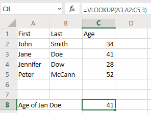
- The value you want to look up is "Jane", which is at cell "A3"
- The range of data you want to search, which is "A2:C5"
- Which column contains the value you want to retrieve? The "Age" is column C, so this argument is 3.
- The 4th argument is optional and we just ignore it for now.
=VLOOKUP(A3, A2:C5, 3)
Below is the result.
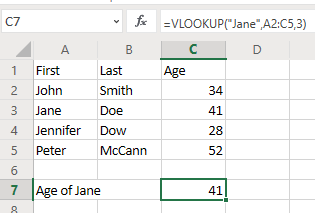
For the value you want to look up, it does not have to be a cell location such as "A3", it can also be an actual value such as "Jane". You can also look up Jane's age this way:
Below is the result.
For the value you want to look up, it does not have to be a cell location such as "A3", it can also be an actual value such as "Jane". You can also look up Jane's age this way:
=VLOOKUP("Jane", A2:C5, 3)
What will happen if we want to retrieve a name which is not on the list? Suppose we try to find Susan's age, while Susan is not on the list. The formula is:
=VLOOKUP("Susan", A2:C5, 3)
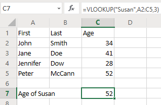
It returns a value of 52, which is obviously wrong, since Susan is not on the list at all. What happened? The VLOOKUP function used approximate matching and it returns the age of Peter as Susan's age.
To solve the problem, we should use the "Exact match" option. So we set the 4th argument to FALSE.
What will happen if we want to retrieve a name which is not on the list? Suppose we try to find Susan's age, while Susan is not on the list. The formula is:
=VLOOKUP("Susan", A2:C5, 3)
It returns a value of 52, which is obviously wrong, since Susan is not on the list at all. What happened? The VLOOKUP function used approximate matching and it returns the age of Peter as Susan's age.
To solve the problem, we should use the "Exact match" option. So we set the 4th argument to FALSE.
=VLOOKUP("Jane", A2:C5, 3, FALSE)
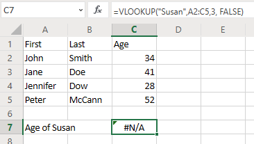
Now it returns an error "#N/A", which means no matching result is found.
Since approximate matching can cause errors which is very hard to identify, we suggest you always used the "Exact match" option in VLOOKUP.
Now it returns an error "#N/A", which means no matching result is found.
Since approximate matching can cause errors which is very hard to identify, we suggest you always used the "Exact match" option in VLOOKUP.
This post is written by Yisong Geng, PhD at Calc LLC. If you need tutoring or development services with Excel, please contact us.
Comments
Post a Comment